Introduction to Federated Learning
It’s Day 1 of the #30DaysOfFLCode Challenge by OpenMined 🥳!
Today I went through an introductory tutorial on Federated Learning by DeepLearning.AI and Flower Labs: Intro to Federated Learning.
Let’s quickly learn a few concepts ⬇️.
Introduction 📉
Why is federated learning needed?
-
Llama-3 is trained on 15 trillion tokens which happens to be very close to the amount of publicly available data. According to a study, we will run out of new publicly available data to further train our models by 2026. In contrast, about 150 trillion tokens are expected to be present in all of the private data globally (e.g., in text messages and emails). This data is not freely accessible for model training.
-
All the data is naturally distributed across industries, geographic locations, devices. For e.g.,
- tons of medical data is distributed among different hospitals.
- individual data is distributed amongst mobile, laptop, home assistants, etc.
Traditional data science methods require all the data to be centrally placed during training. Collecting more data doesn’t work for multiple reasons:
- Sensitive data: Data can be either sensitve or bound by regulations barring it from being used/moved freely.
- Data volume: It can be huge which might cause constraints on storage and computation.
- Practicality: It might not be feasible to collect a lot of data often.
To address these issues, AI models started to shift to a decentralized approach, and a new concept called “federated learning” has emerged.
Federated learning (often referred to as collaborative learning) is a decentralized approach to training machine learning models. It brings the training process to the data than data to the training. It doesn’t require an exchange of data from clients to centralised servers. Organizations retain full control over their data.
A few examples of where its used:
-
Global model for anti-money laundering model: Build a global model to detect money-laundering activity using the customer transcations in USA and EU without moving the data from their respective geographic locations. This makes sure the respective data regulations are followed without compromising model training.
-
Google GBoard on Android: A popular example wherein it is deployed on millions of edge devices to predict the next word based on each user’s data pattern. The model uses FL to learn accurate predictions without needing the data of each user.
Bad Generalization Capabilities due to lack of Complete Data Distribution
Say 3 people have 3 different data distributions of the MNIST dataset each with a few digits missing.
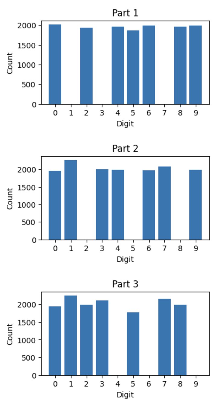
By training 3 different models on the these datasets, we observe the average accuracy of all 3 models to be ~67%. Morevover, the accuracy on specifically the missing data for each model is 0%. This is not a good performing model at all - and in fact a very real challenge.
Model 1->
  Test Accuracy on all digits: 0.6570,
  Test Accuracy on [1,3,7]: 0.0000

Model 2->
  Test Accuracy on all digits: 0.6876,
  Test Accuracy on [2,5,8]: 0.0000

Model 3->
  Test Accuracy on all digits: 0.6848,
  Test Accuracy on [4,6,9]: 0.0000
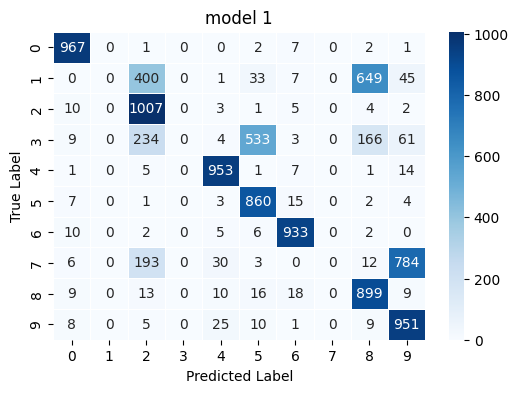
Clearly, the models perform very bad on data it has never seen.
Thus, we’ll now see a big advantage of FL is that all parties can learn from each others data without compromising any private data leakage between them.
Federated Learning Process
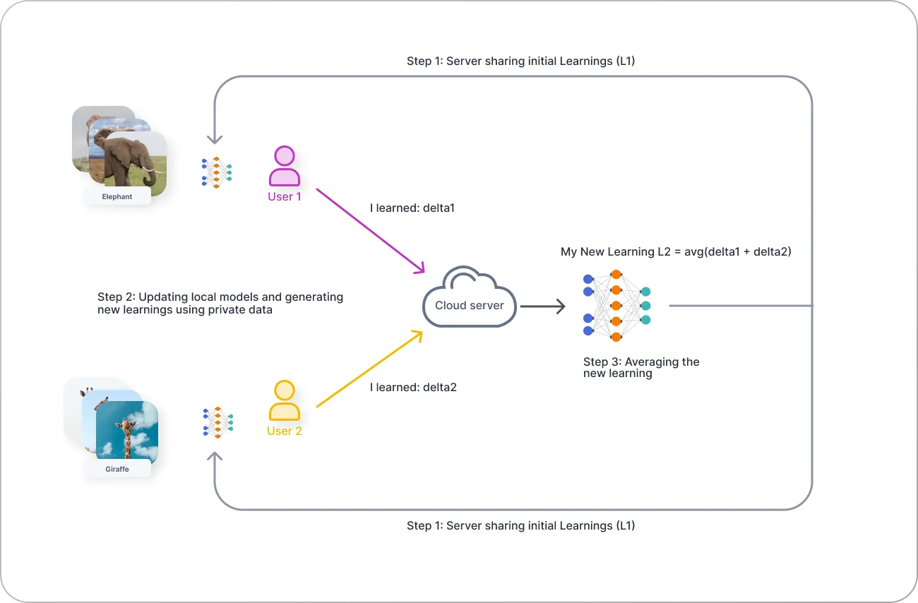
Algorithm
-
Initialization: Server initializes the global model.
- Communication Round: For each round:
- Server sends the global model to the participating clients.
- Each client receives the global model.
- Client Training and Model Update: For each participating client:
- Client trains the received model on its local dataset
- usually for 1-2 epochs.
- overfitting the model on 1 client is bad for the process.
- Client sends its locally updated model to the server.
- Client trains the received model on its local dataset
-
Model Aggregation: Server aggregates the updated models received from all the clienrs using an Aggregating strategy (e.g., FedAvg).
- Convergence Check:
- If convergence critiria is met, end the FL process.
- If not, procedd to the nect communication round (step 2).
Implement using Flower
- Download relevant data.
from flwr.client import Client, ClientApp, NumPyClient
from flwr.common import ndarrays_to_parameters, Context
from flwr.server import ServerApp, ServerConfig
from flwr.server import ServerAppComponents
from flwr.server.strategy import FedAvg
from flwr.simulation import run_simulation


# download mnist dataset
trainset = datasets.MNIST(
    "./MNIST_data/", download=True, train=True, transform=transform
)

# split into 3 different parts to simulate different clients
total_length = len(trainset)
split_size = total_length // 3
torch.manual_seed(42)
part1, part2, part3 = random_split(trainset, [split_size] * 3)

part1 = exclude_digits(part1, excluded_digits=[1, 3, 7])
part2 = exclude_digits(part2, excluded_digits=[2, 5, 8])
part3 = exclude_digits(part3, excluded_digits=[4, 6, 9])

train_sets = [part1, part2, part3]

# Common testset
testset = datasets.MNIST(
    "./MNIST_data/", download=True, train=False, transform=transform
)

testset_137 = include_digits(testset, [1, 3, 7])
testset_258 = include_digits(testset, [2, 5, 8])
testset_469 = include_digits(testset, [4, 6, 9])
- Define the following functions.
-
set_weights: each client uses it to set the global params to the individual model. -
get_weights: each client retrieves the model weight after individual training and returns to server.
-
# Sets the parameters of the model
def set_weights(net, parameters):
    params_dict = zip(net.state_dict().keys(), parameters)
    state_dict = OrderedDict(
        {k: torch.tensor(v) for k, v in params_dict}
    )
    net.load_state_dict(state_dict, strict=True)

# Retrieves the parameters from the model
def get_weights(net):
    ndarrays = [
        val.cpu().numpy() for _, val in net.state_dict().items()
    ]
    return ndarrays
- Create a
FlowerClientto train and evaluate each client model. Flower callsclient_fnwhenever it needs an instance of one particular client to call fit or evaluate.
class FlowerClient(NumPyClient):
    def __init__(self, net, trainset, testset):
        self.net = net
        self.trainset = trainset
        self.testset = testset

    # Train the model
    def fit(self, parameters, config):
        set_weights(self.net, parameters)
        train_model(self.net, self.trainset)
        return get_weights(self.net), len(self.trainset), {}

    # Test the model
    def evaluate(self, parameters: NDArrays, config: Dict[str, Scalar]):
        set_weights(self.net, parameters)
        loss, accuracy = evaluate_model(self.net, self.testset)
        return loss, len(self.testset), {"accuracy": accuracy}


# Client function
def client_fn(context: Context) -> Client:
    net = SimpleModel() # initialise a model for each client
    partition_id = int(context.node_config["partition-id"])
    client_train = train_sets[int(partition_id)] # provide a training set to each client
    client_test = testset
    return FlowerClient(net, client_train, client_test).to_client()

client = ClientApp(client_fn)
- Define an aggregation strategy on server side - here we use
FedAvg.
net = SimpleModel()
params = ndarrays_to_parameters(get_weights(net))

def server_fn(context: Context):
    strategy = FedAvg(
        fraction_fit=1.0, # fit on 100% of the clients
        fraction_evaluate=0.0, # evaluate on 0 clients
        initial_parameters=params,
        evaluate_fn=evaluate, # custom function to calculate accuracy after each epoch of training.
    )
    config=ServerConfig(num_rounds=3) # no. of communication rounds.
    return ServerAppComponents(
        strategy=strategy,
        config=config,
    )

# instantiate the server
server = ServerApp(server_fn=server_fn)
- Run a simulation for FL.
# Initiate the simulation passing the server and client apps
# Specify the number of super nodes that will be selected on every round
run_simulation(
 server_app=server,
 client_app=client,
 num_supernodes=3,
 backend_config=backend_setup,
)
Output:
INFO :      Starting Flower ServerApp, config: num_rounds=3, no round_timeout
INFO :
INFO :      [INIT]
INFO :      Using initial global parameters provided by strategy
INFO :      Evaluating initial global parameters
INFO :      test accuracy on all digits: 0.1267
INFO :      test accuracy on [1,3,7]: 0.2275
INFO :      test accuracy on [2,5,8]: 0.1201
INFO :      test accuracy on [4,6,9]: 0.0380
INFO :
INFO :      [ROUND 1]
INFO :      configure_fit: strategy sampled 3 clients (out of 3)
INFO :      aggregate_fit: received 3 results and 0 failures
INFO :      test accuracy on all digits: 0.8546
INFO :      test accuracy on [1,3,7]: 0.9477
INFO :      test accuracy on [2,5,8]: 0.7771
INFO :      test accuracy on [4,6,9]: 0.7823
INFO :      configure_evaluate: no clients selected, skipping evaluation
INFO :
INFO :      [ROUND 2]
INFO :      configure_fit: strategy sampled 3 clients (out of 3)
INFO :      aggregate_fit: received 3 results and 0 failures
INFO :      test accuracy on all digits: 0.9507
INFO :      test accuracy on [1,3,7]: 0.9619
INFO :      test accuracy on [2,5,8]: 0.9275
INFO :      test accuracy on [4,6,9]: 0.9464
INFO :      configure_evaluate: no clients selected, skipping evaluation
INFO :
INFO :      [ROUND 3]
INFO :      configure_fit: strategy sampled 3 clients (out of 3)
INFO :      aggregate_fit: received 3 results and 0 failures
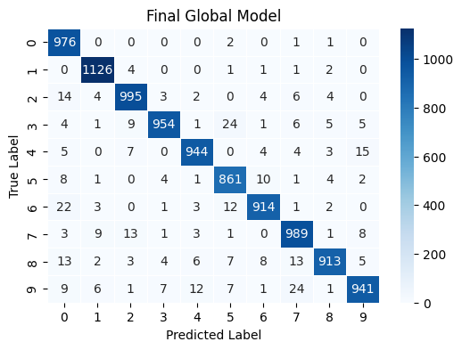
INFO :      test accuracy on all digits: 0.9613
INFO :      test accuracy on [1,3,7]: 0.9672
INFO :      test accuracy on [2,5,8]: 0.9555
INFO :      test accuracy on [4,6,9]: 0.9491
We see that after 3 rounds of FL training, the accuracies of each model is close to 95% on the test set. This is a massive increase from 0% as seen before!**
Tuning
There are multiple components in the FL process that can be tuned:
- Server side:
- client selection: which clients will participate in each round
- client configuration: hyperparameters to use by each client for each round
- hyperparameter tuning
- result aggregation: methods to aggregate model weights on server side
- QFedAvg
- FedAdam
- Vanilla FedAvg
- DP FedAvg
- Client-side:
- preprocessing of weights before applying to the model
- local-training methodology
- post processing of weights before sending back to server
Privacy in federated learning
FL is a data minimization solution. It prevents direct access to the data. However, an adversary can be present on any stage of an FL process.
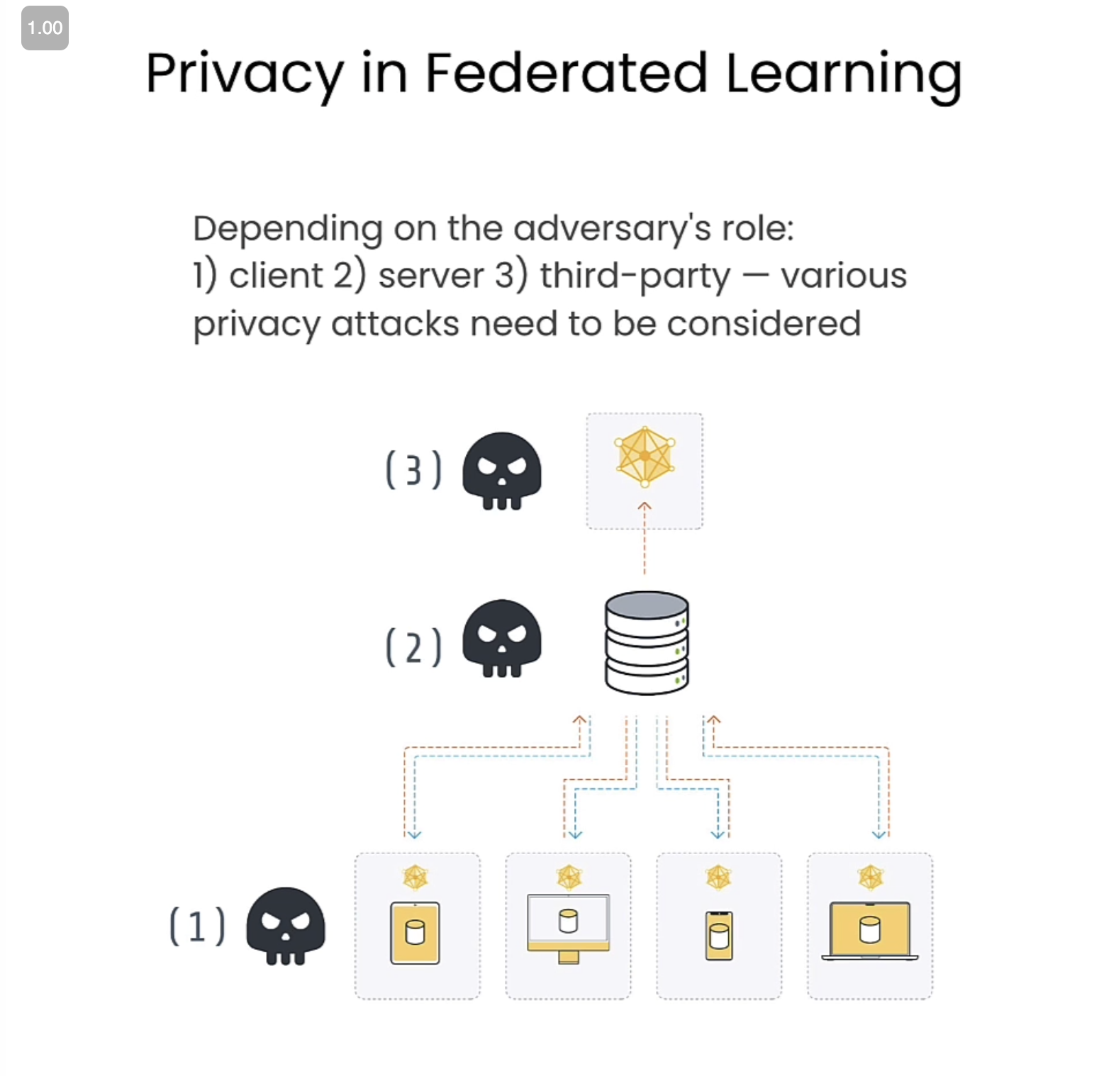
These adversaries have the objective of leaking private data of one of the clients using targetted attacks.
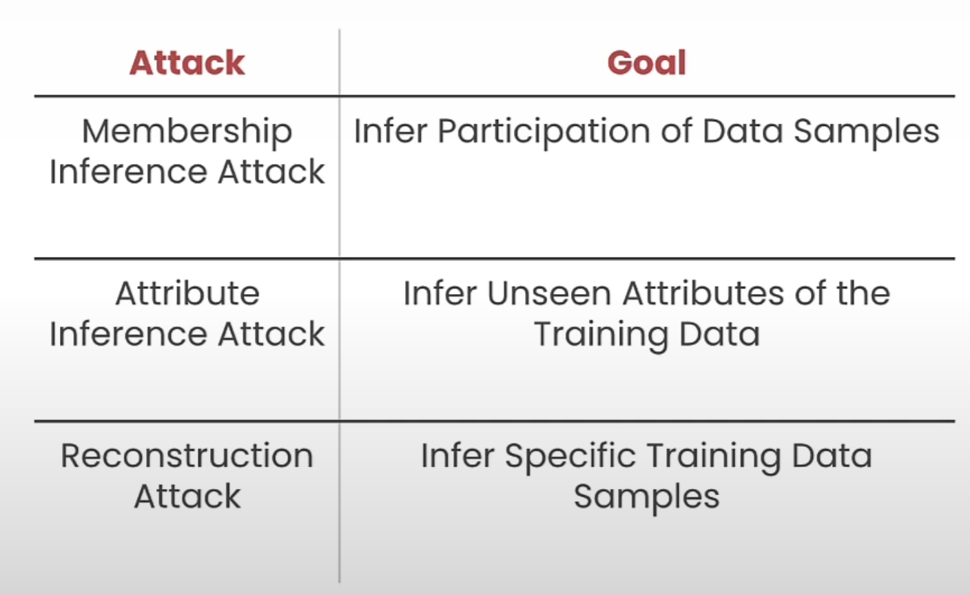
Therefore, many Privacy Enhancing Techniques (PETs) have been introduced to preserve the sensitive data of individuals from leaking in the case of an adversarial attack. One such is called Differential Privacy.
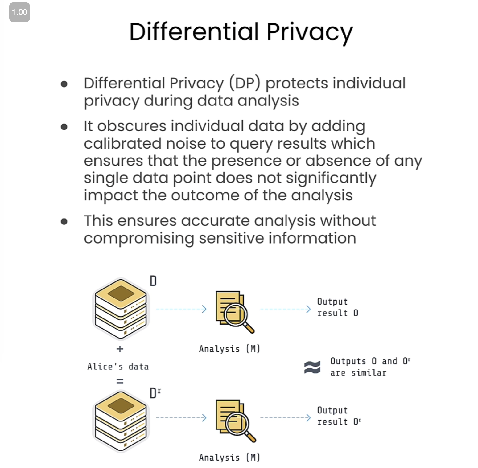
Differential Privacy in FL
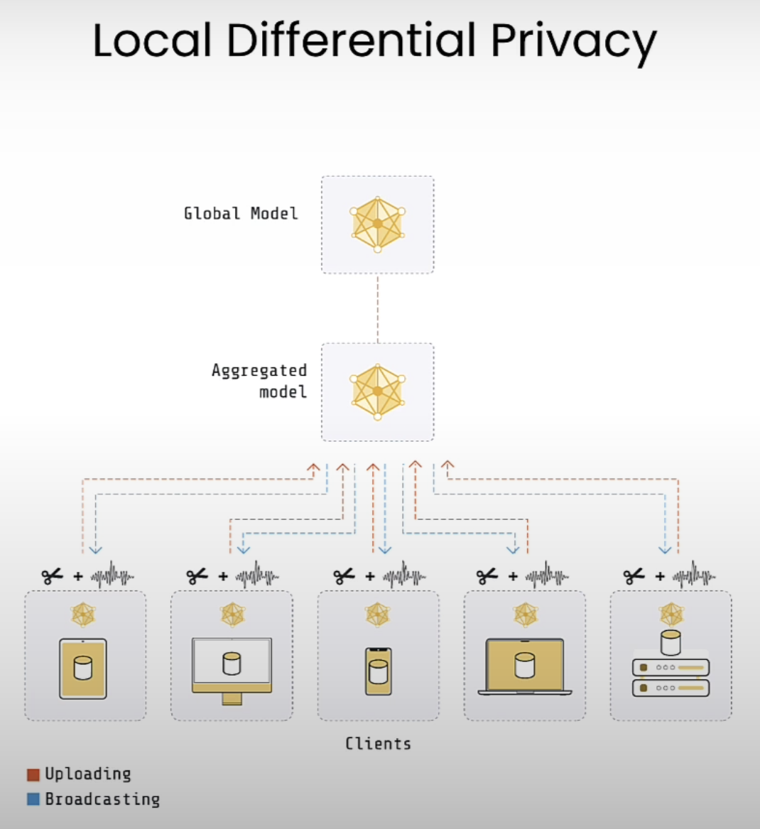
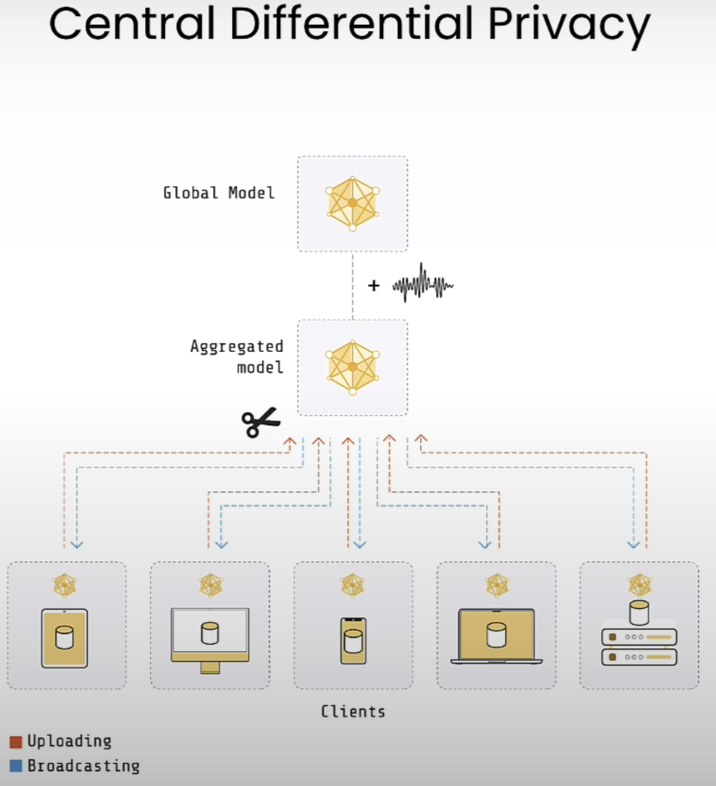
DP in FL aims to protect the privacy of client’s data. Depending in the intended level of privacy, utility, and the role of the adversary, it can be categorized into variants suh as central and local.
This involves 2 steps:
-
Clipping: Bounds the sensitivity and mitigates the impact of outliers.
-
Noising: Adds a calibrated noise to make the output statiscally indistinguishable.
Let’s implement it using flower.
from flwr.server.strategy import (
    DifferentialPrivacyClientSideAdaptiveClipping,
    FedAvg,
)

def server_fn(context: Context):
    fedavg_without_dp = FedAvg(
        fraction_fit=0.6,
        fraction_evaluate=1.0,
        initial_parameters=params,
    )

    # Client side will clip the updates
    fedavg_with_dp = DifferentialPrivacyClientSideAdaptiveClipping(
        fedavg_without_dp,  # <- wrap the FedAvg strategy
        noise_multiplier=0.3, # Server will add noise after aggregation
        num_sampled_clients=6,
    )

    # Adjust to 50 rounds to ensure DP guarantees hold
    # with respect to the desired privacy budget
    config = ServerConfig(num_rounds=5)

    return ServerAppComponents(
        strategy=fedavg_with_dp,
        config=config,
    )
That is all for today folks! Blogging + learning is a long process haha, but I’m glad I learnt a bunch today!
See you tomorrow :D
References
[1] https://learn.deeplearning.ai/courses/intro-to-federated-learning/
Enjoy Reading This Article?
Here are some more articles you might like to read next: